PDE-based modelling of Covid-19 infections
The developed model is a paradigm shift in mathematical modeling of infectious diseases.
This modeling framework introduces a multi-dimensional equation to predict the spread of pandemics with insights into the severity of infection, duration of infection, population age etc. Such insightful predictions are key for planning lockdown/unlock strategies and public health policies such as quarantine rules, hospital beds, health insurance and vaccination/treatment scheduling. Moreover, these insights can be used to formulate science-informed policy to revive normalcy in the world, especially from the disruption induced by Covid-19. A detailed description of the predictive modeling framework can be found here. arXiv:2006.15336 .
Model predictions updated on June 18, 2020 . For previous results click here (May 28, 2020) and here (May 3, 2020).
Key Observations
- The recovery rate has increased since May 3, 2020 and consequently reduced new infections. It emphasises the importance of appropriate medical care and timely quarantine.
- Among all measures, contact tracing, quarantine and social distancing are key to contain the spread in the absence of vaccine.
- One or two day lockdown per week (e.g., Sunday, Sunday & Wednesday etc) with complete compliance along with adequate social distancing during other days is effective to reduce the spread.
- Proposed model can be used to predict region-wise and age-wise COVID-19 spread accurately, and consequently it can be used to frame policies on periodic lockdown, staggered opening of educational institutions and public facilities.
Choose India/State/UT*
Chart loading
Select
Duration
Duration
(Click on the above square buttons to remove/add a plot.
Use the time slider to adjust time period.)
Computational Model
- Data* between 23 Mar and 18 June, 2020 is used partially to tune the parameters of the data-driven model. These results are current as of June 18, 2020.
- State-wise results are computed with the parameters of national trend to compare the performance of the respective state with the national trend. See Discussion for interpretation.
- Quarantine of Active Cases so as to prevent new infections is the key to contain the pandemic. An adaptive quarantine function in our model ensures that infected population is quarantined based on their infection level (showing symptoms) and based on latest published literature on how the infection spreads from infected population.
- The severity of the infection is taken into consideration while modeling the infectious death rate function (see the rate functions in the model).
- Differnt scenarios are modeled based on anticipated individual behavior (social distancing, hygiene practice, compliance to government rules etc.), government policies (quarantine rules, lockdown rules etc.).
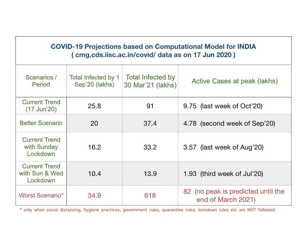
- Current Trend follows business as usual assuming further relaxation to lockdown rules. Better and Worse Scenarios assume better and worse compliance. Weekly lockdown models the impact of a complete lockdown on Sunday and Sunday & Wednesday respectively.
Observations
- Current Trend: Hits a peak of 9.75 lakh ‘Active Cases’ in the last week of October 2020. Further, there will be around 2.1 lakh ‘Active Cases’, 4.5 lakh deaths and 91 lakh toal cases at the end of March 2021.
- Better Scenario: Hits a peak of 4.78 lakh 'Active Cases' in the second week of September 2020. Further, there will be around 14.2 thousand ‘Active Cases’, 1.88 lakh deaths and 37.4 lakh total cases at the end of March 2021.
- Worse Scenario: No peak is predicted until end of March 2021. There will around 82 lakh ‘Active Cases’ still growing, 28 lakh deaths and 6.18 crore total cases at the end of March 2021.
- Current Trend with Sunday Lockdown:Hits a peak of 3.57 lakh ‘Active Cases’ in the last week of August 2020. Further, there will be around 30.2 thousand ‘Active Cases’, 1.67 lakh deaths and 33.2 lakh total cases at the end of March 2021.
- Current Trend with Sun & Wed Lockdown: Hits a peak of 1.93 lakh Active Cases in the third week of July 2020. Further, there will around 2.8 thousand ‘Active’ Cases, 70.3 thousand deaths and 13.9 lakh total cases at the end of March 2021.
Discussion
- In order to achieve and follow the Current Trend prediction for the next one year, people should maintain the same or even better level of social distancing as maintained during 23 Mar - 18 June 2020. It is assumed that awareness increases with time and there is more compliance of social distancing and other norms. Also, we anticipate that more members of the susceptible population improve their hygiene practice and immunity levels.
- Until the development of vaccines, social distancing and other practices to reduce interaction among people (such as avoiding mass gathering etc.) are the key tools to contain the spread of COVID-19. As such, public awareness of these practices through several modes (advertisements through TV, radios, new papers, social media, etc.) is crucial.
- The Better Scenario and Worse Scenario model the infection spread when there is better and worse compliance of social distancing and other norms among susceptible population.
- Short, periodic (e.g., one or two days per week) lockdown with complete compliance to stay at home and avoid interaction helps reduce infection. This must be combined with increased social distancing and quarantining of suspected population during non-lockdown phases. The ‘Sunday Lockdown’ and ‘Sun & Wed Lockdown’ scenarios model these strategies.
- Since this is an active situation with regular ongoing interventions and policy changes from State and Central governments, we do not predict each state individually and the state numbers have to be interpreted as follows.
- In each scenario, the state numbers are computed with the national parameters. This is done to compare the actual data of the state with the national trend.
- For example, Kerala, Karnataka, Uttar Pradesh (and others) have done better than the national trend. Whereas, Maharashtra, Tamil Nadu, Madhya Pradesh (and others) have done worse than the national trend. Some states such as Rajasthan, Andhra Pradesh (and others) have done similar to the national trend.
- The forecast range of all predicted scenarios (some shown here, others not shown) can be viewed by enabling the uncertainty region in the time series plots. The region may be interpreted as the "Confidence Interval" for the forecast numbers.
State Performance Compared to National Trend
Team
- Lead: Prof. Sashikumaar Ganesan and Prof. Deepak Subramani CDS, IISc Bangalore, India
- Email: sashi@iisc.ac.in, deepakns@iisc.ac.in
- Members: Chris Francis
High-Dimensional Population Balance Model
Key Features
- A six-dimensional population balance predictive computational model for an epidemic.
- Unlike the existing (Compartment or Network) models, proposed model predicts the distribution of infected population across the region, the age of the infected people, the day since infection, and the severity of infection, over a period of time.
- Incorporates the immunity, pre-medical history, effective treatment, point-to-point movement of infected population (e.g., by air, train etc), interactivity (community spread), hygiene and the social distancing of the population.
- Finite element operator-splitting scheme for the high-dimensional PDE.
A detailed description of the predictive modeling framework can be found here. arXiv:2006.15336
Note: Double-click/double-tap on an equation to zoom.
Population Balance Model
Let $T_\infty$ be a given final time and $\Omega:=\Omega_x\otimes\Omega_\ell$ be the computational domain of interest. Here, $\Omega_x\subset\mathbb{R}^2$ is the spatial domain defining the geographical region of interest and $\Omega_\ell:=L_v\times L_d\times L_a$ is an internal domain, where $L_v=[0, 1]$ denotes the Covid-19 infection severity interval, $L_d=[0,d_{\max}]$ denotes the time interval since contracting the disease, and $L_a=[0, 1]$ denotes the non-dimensional age interval with the non-dimensionalization constant being 125 years. The infection index $\ell_v\in L_v$ quantifies the severity of the population being infected by Covid-19. Specifically, the population with infection index $\ell_v=0$ has recovered completely from Covid-19, with $\ell_v = 1$ has died due it, with $\ell_v\ge v_{\rm sym}$ shows symptoms and those with $\ell_v\le v_{\rm sym}$ are asymptomatic. The time since contracting the disease index $\ell_d\in L_d$ quantifies the time since a population has been exposed to and contracted the disease. Specifically, the population that just contracted the disease has $\ell_d=0$. Typically, a person is asymptomatic until they reach $\ell_v=v_{\rm sym}$, and the duration elapsed $\ell_d$ is the incubation period in which the disease is sub-clinical and that population is actively spreading the disease. After recovery, a population doesn't necessarily go to $\ell_v=0$, rather they reach $\ell_v\le v_{\rm reco}$.
... Let $I(t,x,\ell_v,\ell_d,\ell_a)$ be the size distribution function of the infected population. To describe the evolution of the active infected population size distribution, we propose the population balance equation \begin{equation}\label{model} \begin{array}{rcll} \displaystyle\frac{\partial I}{\partial t} + \nabla_x\cdot({\bf u} I) +\nabla_\ell\cdot({\bf G} I) +CI &=& F \quad &{\rm in } \quad (0,T_\infty]\times\Omega_x\times\Omega_\ell \,,\\ I(t,x,\ell) &=&g_n &{\textrm in } \quad (0,T_\infty]\times\partial\Omega^{-}_{ x}\times L_v\times L_d\times L_a\,\\ I(t,\mathbf{x},\ell_v,0,\ell_a) & =& B_{\rm nuc} \quad &{\rm in } \quad (0,T_\infty]\times\Omega_{x}\times L_v\times L_a \,,\\ I(t,\mathbf{x},0,\ell_d>0,\ell_a) & =& 0 \quad &{\rm in } \quad (0,T_\infty]\times\Omega_{x}\times L_d\times L_a \,,\\ I(0,x,\ell) & =& I_0 &{\rm in } \quad \Omega_{x}\times\Omega_\ell \,. \end{array} \end{equation} Here, ${\bf u}$ denotes the advection vector that quantifies the spatial movement of the population in a differential neighbourhood of $\Omega_{x}$, $f(t,x,\ell_a)$ denotes the net addition of an infected population into $\Omega_{\rm x}$ from outside, ${\bf n}$ is the outward unit normal vector to $\Omega_x$, $\partial{\Omega}^{-}:= \{x \in \partial{\Omega_{x}} \ |~ {\bf u}\cdot {\bf n} <0 \ \}$, $g_n$ is the flux that quantifies the net addition of an infected population into $\Omega_{\rm x}$ from outside (the spatial movement of the population across the border of the domain $\partial\Omega_{\rm x}$), and $I_0$ is the initial distribution of infected population. Further, $ {\bf G} = (G_{\ell_v}, G_{\ell_d}, G_{\ell_a})^T $ is the internal growth vector. Here, the Covid-19 infection severity growth rate in an infected population is defined by \begin{equation} G_{\ell_v} = \frac{d \ell_v}{d t} = G_{\ell_v}(\ell_a, \beta, \gamma(\ell_a), \alpha(x) ), \end{equation} where $\beta$ is the immunity of the infected population, $\gamma$ is the pre-medical history of the infected population and $\alpha$ is the effective treatment index. Additionally, the time since infection index has a growth rate \begin{equation} G_{\ell_d} = \frac{d \ell_d}{d t} = 1\,. \end{equation} Moreover, the change of age of the active, infected population can be modelled through the growth rate \begin{equation} G_{\ell_a} = \frac{d \ell_a}{d t}. \end{equation} Nevertheless, the influence will be negligible when the study is performed for a short duration $(0, T_\infty]$, and thereby may be ignored. $G_{\ell_v}$ is the growth function of the Covid-19 infection index $l_v$, We next rate term \begin{equation} C = C_R + C_{ID}, \end{equation} where $C_R(t,\mathbf{x},\ell_v,\ell_d,\ell_a)$ is a recovery rate function that quantifies the rate of recovery of the population from Covid-19 and $C_{ID}(t,\mathbf{x},\ell_v,\ell_d,\ell_a)$ is the Covid-19 death rate. We also define a source term $F = C_T(t,\mathbf{x},\ell_v,\ell_d,\ell_a)$ that quantifies the point-to-point movement of infected population (e.g., by air, train etc) within $\Omega_x$ not explained by ${\bf u}$ and the source/sink of infected population travelled by air into $\Omega_x$ not explained by $g_n$. Moreover, $C_T$ and ${\bf u}$ need to be defined in such a way that the net internal movement of infected population within $\Omega_{x}$ is conserved. Moreover $B_{\rm nuc}$ is the nucleation function that quantifies how a susceptible population becomes infected and it is defined by \begin{equation} B_{\rm nuc}(t,\mathbf{x},\ell_v,\ell_a) = B_{\rm nuc}\left(C_Q, \ell_a, \sigma, H, S_D, N_S(t), N_Q(t) I\right), \qquad \forall ~\ell_v,\ell_a\in L_v\times L_a. \end{equation} Here, $C_Q(t,\mathbf{x},\ell_v,\ell_d,\ell_a)$ is a quarantine rate that quantifies the removal of people into a quarantine facility, $\sigma\in[0,1]$ is the interactivity index, $H\in[0,1]$ is the hygiene index, $S_D\in[0,1]$ is the social distancing index. Finally, the total population $N(t)$ at a given time $t\in(0,T_\infty]$ is defined by \begin{align*} N(t) &= N_S(t) + N_R(t) + N_I(t) +N_Q(t) - N_{ID}(t) - N_D(t), \\ N_I(t) &= \int_{\Omega} I(t,\mathbf{x},\ell_v,\ell_d,\ell_a)\,d\Omega\,,\\ N_Q(t) &= \int_{\Omega} \gamma_Q(t,\mathbf{x},\ell_v,\ell_d,\ell_a)I(t,\mathbf{x},\ell_v,\ell_d,\ell_a) \,dx\,d\ell\,,\\ N_{R}(t) &= \int_{\Omega} C_RI(t,\mathbf{x},\ell_v,\ell_d,\ell_a)\,d\Omega\ \,,\\ N_{ID}(t) &= \int_{\Omega} C_{ID}I(t,\mathbf{x},\ell_v,\ell_d,\ell_a)\,d\Omega \,,\\ N_S(t) &= N(t) - [N_I(t)+N_Q(t)+N_R(t)-N_{ID}(t)-N_D(t)] \,. \end{align*} Here, $N_S$, $N_B$, $N_R$, $N_I$, $N_Q$ $N_{ID}$ and $N_D$ are the number of susceptible, newborn, recovered, asymptomatic/symptomatic infectives, quarantined, infective death and natural death populations, respectively. The population in the interval $(v_{\rm reco},v_{\min})$ has recovered from Covid-19.
... Let $I(t,x,\ell_v,\ell_d,\ell_a)$ be the size distribution function of the infected population. To describe the evolution of the active infected population size distribution, we propose the population balance equation \begin{equation}\label{model} \begin{array}{rcll} \displaystyle\frac{\partial I}{\partial t} + \nabla_x\cdot({\bf u} I) +\nabla_\ell\cdot({\bf G} I) +CI &=& F \quad &{\rm in } \quad (0,T_\infty]\times\Omega_x\times\Omega_\ell \,,\\ I(t,x,\ell) &=&g_n &{\textrm in } \quad (0,T_\infty]\times\partial\Omega^{-}_{ x}\times L_v\times L_d\times L_a\,\\ I(t,\mathbf{x},\ell_v,0,\ell_a) & =& B_{\rm nuc} \quad &{\rm in } \quad (0,T_\infty]\times\Omega_{x}\times L_v\times L_a \,,\\ I(t,\mathbf{x},0,\ell_d>0,\ell_a) & =& 0 \quad &{\rm in } \quad (0,T_\infty]\times\Omega_{x}\times L_d\times L_a \,,\\ I(0,x,\ell) & =& I_0 &{\rm in } \quad \Omega_{x}\times\Omega_\ell \,. \end{array} \end{equation} Here, ${\bf u}$ denotes the advection vector that quantifies the spatial movement of the population in a differential neighbourhood of $\Omega_{x}$, $f(t,x,\ell_a)$ denotes the net addition of an infected population into $\Omega_{\rm x}$ from outside, ${\bf n}$ is the outward unit normal vector to $\Omega_x$, $\partial{\Omega}^{-}:= \{x \in \partial{\Omega_{x}} \ |~ {\bf u}\cdot {\bf n} <0 \ \}$, $g_n$ is the flux that quantifies the net addition of an infected population into $\Omega_{\rm x}$ from outside (the spatial movement of the population across the border of the domain $\partial\Omega_{\rm x}$), and $I_0$ is the initial distribution of infected population. Further, $ {\bf G} = (G_{\ell_v}, G_{\ell_d}, G_{\ell_a})^T $ is the internal growth vector. Here, the Covid-19 infection severity growth rate in an infected population is defined by \begin{equation} G_{\ell_v} = \frac{d \ell_v}{d t} = G_{\ell_v}(\ell_a, \beta, \gamma(\ell_a), \alpha(x) ), \end{equation} where $\beta$ is the immunity of the infected population, $\gamma$ is the pre-medical history of the infected population and $\alpha$ is the effective treatment index. Additionally, the time since infection index has a growth rate \begin{equation} G_{\ell_d} = \frac{d \ell_d}{d t} = 1\,. \end{equation} Moreover, the change of age of the active, infected population can be modelled through the growth rate \begin{equation} G_{\ell_a} = \frac{d \ell_a}{d t}. \end{equation} Nevertheless, the influence will be negligible when the study is performed for a short duration $(0, T_\infty]$, and thereby may be ignored. $G_{\ell_v}$ is the growth function of the Covid-19 infection index $l_v$, We next rate term \begin{equation} C = C_R + C_{ID}, \end{equation} where $C_R(t,\mathbf{x},\ell_v,\ell_d,\ell_a)$ is a recovery rate function that quantifies the rate of recovery of the population from Covid-19 and $C_{ID}(t,\mathbf{x},\ell_v,\ell_d,\ell_a)$ is the Covid-19 death rate. We also define a source term $F = C_T(t,\mathbf{x},\ell_v,\ell_d,\ell_a)$ that quantifies the point-to-point movement of infected population (e.g., by air, train etc) within $\Omega_x$ not explained by ${\bf u}$ and the source/sink of infected population travelled by air into $\Omega_x$ not explained by $g_n$. Moreover, $C_T$ and ${\bf u}$ need to be defined in such a way that the net internal movement of infected population within $\Omega_{x}$ is conserved. Moreover $B_{\rm nuc}$ is the nucleation function that quantifies how a susceptible population becomes infected and it is defined by \begin{equation} B_{\rm nuc}(t,\mathbf{x},\ell_v,\ell_a) = B_{\rm nuc}\left(C_Q, \ell_a, \sigma, H, S_D, N_S(t), N_Q(t) I\right), \qquad \forall ~\ell_v,\ell_a\in L_v\times L_a. \end{equation} Here, $C_Q(t,\mathbf{x},\ell_v,\ell_d,\ell_a)$ is a quarantine rate that quantifies the removal of people into a quarantine facility, $\sigma\in[0,1]$ is the interactivity index, $H\in[0,1]$ is the hygiene index, $S_D\in[0,1]$ is the social distancing index. Finally, the total population $N(t)$ at a given time $t\in(0,T_\infty]$ is defined by \begin{align*} N(t) &= N_S(t) + N_R(t) + N_I(t) +N_Q(t) - N_{ID}(t) - N_D(t), \\ N_I(t) &= \int_{\Omega} I(t,\mathbf{x},\ell_v,\ell_d,\ell_a)\,d\Omega\,,\\ N_Q(t) &= \int_{\Omega} \gamma_Q(t,\mathbf{x},\ell_v,\ell_d,\ell_a)I(t,\mathbf{x},\ell_v,\ell_d,\ell_a) \,dx\,d\ell\,,\\ N_{R}(t) &= \int_{\Omega} C_RI(t,\mathbf{x},\ell_v,\ell_d,\ell_a)\,d\Omega\ \,,\\ N_{ID}(t) &= \int_{\Omega} C_{ID}I(t,\mathbf{x},\ell_v,\ell_d,\ell_a)\,d\Omega \,,\\ N_S(t) &= N(t) - [N_I(t)+N_Q(t)+N_R(t)-N_{ID}(t)-N_D(t)] \,. \end{align*} Here, $N_S$, $N_B$, $N_R$, $N_I$, $N_Q$ $N_{ID}$ and $N_D$ are the number of susceptible, newborn, recovered, asymptomatic/symptomatic infectives, quarantined, infective death and natural death populations, respectively. The population in the interval $(v_{\rm reco},v_{\min})$ has recovered from Covid-19.
Finite Element Approximation
A finite element scheme [1] based on operator splitting [2-5] has been implemented in our in-house (open-source) finite element package to solve the high-dimensional population balance equation.References
- S. Ganesan, L. Tobiska, Finite Elements: Theory and Algorithms, Cambridge IISc Series, Cambridge University Press, 2016.
- S. Ganesan, L. Tobiska, Operator-splitting finite element algorithms for computations of high-dimensional parabolic problems, Appl. Math. Comp. 219 (2013) 6182-6196.
- S. Ganesan, L. Tobiska, An operator-splitting finite element method for the efficient parallel solution of multidimensional population balance systems, Chem. Eng. Sci. 69 (1) (2012) 59-68.
- S. Ganesan, An operator-splitting Galerkin/SUPG finite element method for population balance equations: Stability and convergence, ESAIM: M2AN 46 (2012) 1447-1465.
- P. S. kumar, S. Ganesan, Numerical simulation of nanocrystal synthesis in a microfluidic reactor, Chem. Eng. Sci. 96 (2017) 128-138.
Acknowledgements
- COVID19-India API
- DataMeet/maps
- Members of eXComp group, CDS, IISc Bangalore
- Special thanks to all well wishers and colleagues for the discussion and feedback on our model.
- We thank the Indian Academy of Science Summer Fellowship Program for the support to Chris.
- Deepak wishes to acknowledge DST Inspire and Arcot Ramachandran Young Investigator Awards.
- Sashi wishes to acknowledge SERB and DRDO for the grants that supported development of ParMooN.